10 Things You Need to Know About Statistical Power
This guide will help you assess and improve the power of your experiments. We focus on the big ideas and provide examples and tools that you can use in R.
1 1. What Power Is
Power is the ability to distinguish signal from noise.
The signal that we are interested in is the impact of a treatment on some outcome. Does education increase incomes? Do public health campaigns decrease the incidence of disease? Can international monitoring decrease government corruption?
The noise that we are concerned about comes from the complexity of the world. Outcomes vary across people and places for myriad reasons. In statistical terms, you can think of this variation as the standard deviation of the outcome variable. For example, suppose an experiment uses rates of a rare disease as an outcome. The total number of affected people isn’t likely to fluctuate wildly day to day, meaning that the background noise in this environment will be low. When noise is low, experiments can detect even small changes in average outcomes. A treatment that decreased the incidence of the disease by 1% percentage points would be easily detected, because the baseline rates are so constant.
Now suppose an experiment instead used subjects’ income as an outcome variable. Incomes can vary pretty widely – in some places, it is not uncommon for people to have neighbors that earn two, ten, or one hundred times their daily wages. When noise is high, experiments have more trouble. A treatment that increased workers’ incomes by 1% would be difficult to detect, because incomes differ by so much in the first place.
A major concern before embarking on an experiment is the danger of a false negative. Suppose the treatment really does have a causal impact on outcomes. It would be a shame to go to all the trouble and expense of randomizing the treatment, collecting data on both treatment and control groups, and analyzing the results, just to have the effect be overwhelmed by background noise.
If our experiments are highly-powered, we can be confident that if there truly is a treatment effect, we’ll be able to see it.
2 2. Why You Need It
Experimenters often guard against false positives with statistical significance tests. After an experiment has been run, we are concerned about falsely concluding that there is an effect when there really isn’t.
Power analysis asks the opposite question: supposing there truly is a treatment effect and you were to run your experiment a huge number of times, how often will you get a statistically significant result?
Answering this question requires informed guesswork. You’ll have to supply guesses as to how big your treatment effect can reasonably be, how many subjects will answer your survey, how many subjects your organization can realistically afford to treat.
Where do these guesses come from? Before an experiment is run, there is often a wealth of baseline data that are available. How old/rich/educated are subjects like yours going to be? How big was the biggest treatment effect ever established for your dependent variable? With power analysis, you can see how sensitive the probability of getting significant results is to changes in your assumptions.
Many disciplines have settled on a target power value of 0.80. Researchers will tweak their designs and assumptions until they can be confident that their experiments will return statistically significant results 80% of the time. While this convention is a useful benchmark, be sure that you are comfortable with the risks associated with an 80% expected success rate.
A note of caution: power matters a lot. Negative results from underpowered studies can be hard to interpret: Is there really no effect? Or is the study just not able to figure it out? Positive results from an underpowered study can also be misleading: conditional upon being statistically significant, an estimate from an underpowered study probably overestimates treatment effects. Under powered studies are sometimes based on overly optimistic assumptions; a convincing power analysis makes these assumptions explicit and should protect you from implementing designs that realistically have no chance of answering the questions you want to answer.
3 3. The Three Ingredients of Statistical Power
There are three big categories of things that determine how highly powered your experiment will be. The first two (the strength of the treatment and background noise) are things that you can’t really control – these are the realities of your experimental environment. The last, the experimental design, is the only thing that you have power over – use it!
Strength of the treatment. As the strength of your treatment increases, the power of your experiment increases. This makes sense: if your treatment were giving every subject $1,000,000, there is little doubt that we could discern differences in behavior between the treatment and control groups. Many times, however, we are not in control of the strength of our treatments. For example, researchers involved in program evaluation don’t get to decide what the treatment should be, they are supposed to evaluate the program as it is.
Background noise. As the background noise of your outcome variables increases, the power of your experiment decreases. To the extent that it is possible, try to select outcome variables that have low variability. In practical terms, this means comparing the standard deviation of the outcome variable to the expected treatment effect size — there is no magic ratio that you should be shooting for, but the closer the two are, the better off your experiment will be. By and large, researchers are not in control of background noise, and picking lower-noise outcome variables is easier said than done. Furthermore, many outcomes we would like to study are inherently quite variable. From this perspective, background noise is something you just have to deal with as best you can.
Experimental Design. Traditional power analysis focuses on one (albeit very important) element of experimental design: the number of subjects in each experimental group. Put simply, a larger number of subjects increases power. However, there are other elements of the experimental design that can increase power: how is the randomization conducted? Will other factors be statistically controlled for? How many treatment groups will there be, and can they be combined in some analyses?
4 4. Key Formulas for Calculating Power
Statisticians have derived formulas for calculating the power of many experimental designs. They can be useful as a back of the envelope calculation of how large a sample you’ll need. Be careful, though, because the assumptions behind the formulas can sometimes be obscure, and worse, they can be wrong.
Here is a common formula used to calculate power:1
\(\beta\) is our measure of power. Because it’s the probability of getting a statistically significant result, β will be a number between 0 and 1.
\(\Phi\) is the CDF of the normal distribution, and \(\Phi^{-1}\) is its inverse. Everything else in this formula, we have to plug in:
\(\mu_t\) is the average outcome in the treatment group. Suppose it’s 65.
\(\mu_c\) is the average outcome in the control group. Suppose it’s 60.
Together, assumptions about μt and μc define our assumption about the size of the treatment effect: 65-60= 5.
\(\sigma\) is the standard deviation of outcomes. This is how we make assumptions about how noisy our experiment will be — one of the assumptions we’re making is that sigma is the same for both the treatment and control groups. Suppose \(\sigma=20\)
\(\alpha\) is our significance level – the convention in many disciplines is that α should be equal to 0.05. \(N\) is the total number of subjects. This is the only variable that is under the direct control of the researcher. This formula assumes that every subject had a 50/50 chance of being in control. Suppose that \(N=500\).
Working through the formula, we find that under this set of assumptions, \(β = 0.80\), meaning that we have an 80% chance of recovering a statistically significant result with this design. Click here for a google spreadsheet that includes this formula. You can copy these formulas directly into Excel. If you’re comfortable in R, here is code that will accomplish the same calculation.
In addition, EGAP has created a power calculator Shiny app, which you can access here.
5 5. When to Believe Your Power Analysis
From some perspectives the whole idea of power analysis makes no sense. You want to figure out the size of some treatment effect but first you need to do a power analysis which requires that you already know your treatment effect and a lot more besides.
So in most power analyses you are in fact seeing what happens with numbers that are to some extent made up. The good news is that it is easy to find out how much your conclusions depend on your assumptions: simply vary your assumptions and see how the conclusions on power vary.
This is most easily seen by thinking about how power varies with the number of subjects. A power analysis that looks at power for different study sizes simply plugs in a range of values in for N and seeing how β changes.
Using the formula in section 4, you can see how sensitive power is to all of the assumptions: Power will be higher if you assume the treatment effect will be larger, or if you’re willing to accept a higher alpha level, or if you have more or less confidence in the noisiness of your measures.2
6 6. How to Use Simulation to Estimate Power
Power is a measure of how often, given assumptions, we would obtain statistically significant results, if we were to conduct our experiment thousands of times. The power calculation formula takes assumptions and return an analytic solution. However, due to advances in modern computing, we don’t have to rely on analytic solutions for power analysis. We can tell our computers to literally run the experiment thousands of times and simply count how frequently our experiment comes up significant.
The code block below shows how to conduct this simulation in R using DeclareDesign.
Code
library(DeclareDesign)library(knitr)library(kableExtra)set.seed(1234)# Set up sample size and treatment effectN <-500tau <-0.2design <-# First, specify a model that generates baseline data for the units in the studydeclare_model(N = N,X =rep(c(0,2), each = N/2),U =rnorm(N),potential_outcomes(Y~tau*Z + X + U)) +# Second, specify the inquirydeclare_inquiry(ATE =mean(Y_Z_1 - Y_Z_0)) +# Third, set the data strategydeclare_assignment(Z =complete_ra(N = N, m = N/2)) +declare_measurement(Y =reveal_outcomes(Y ~ Z)) +# Finally, set the estimatorsdeclare_estimator(Y ~ Z, inquiry ="ATE", .method = lm_robust, label ="Simple") +declare_estimator(Y ~ Z + X, inquiry ="ATE", .method = lm_robust, label ="Covariate Adjusted")# Specify an alpha level to test for the power of the designalpha <-0.05study_diagnosands <-declare_diagnosands(power =mean(p.value <= alpha))#One diagnostic rundiag <-diagnose_design(design, diagnosands = study_diagnosands, sims=500)#specify sample sizes of interestpossible.ns <-seq(from=100, to=2000, by=40)#Redesign for different sample sizes between 100 and 2000 by 40designN <-redesign(design, N =seq(from=100, to=2000, by=40))#Run power analysis on each designdiagnose <-diagnose_design(designN, diagnosands = study_diagnosands, sims =500)#store dataset of power analysisplotdf <- diagnose$diagnosands_df#print power for the simple regression approach (first 5 rows)kable_styling(kable(head(plotdf[c(plotdf$estimator=="Simple"), c(2,7)]), row.names = F))
N
power
100
0.110
140
0.132
180
0.174
220
0.154
260
0.184
300
0.214
The code for this simulation and others is available here. Simulation is a far more flexible, and far more intuitive way to think about power analysis. Even the smallest tweaks to an experimental design are difficult to capture in a formula (adding a second treatment group, for example), but are relatively straightforward to include in a simulation.
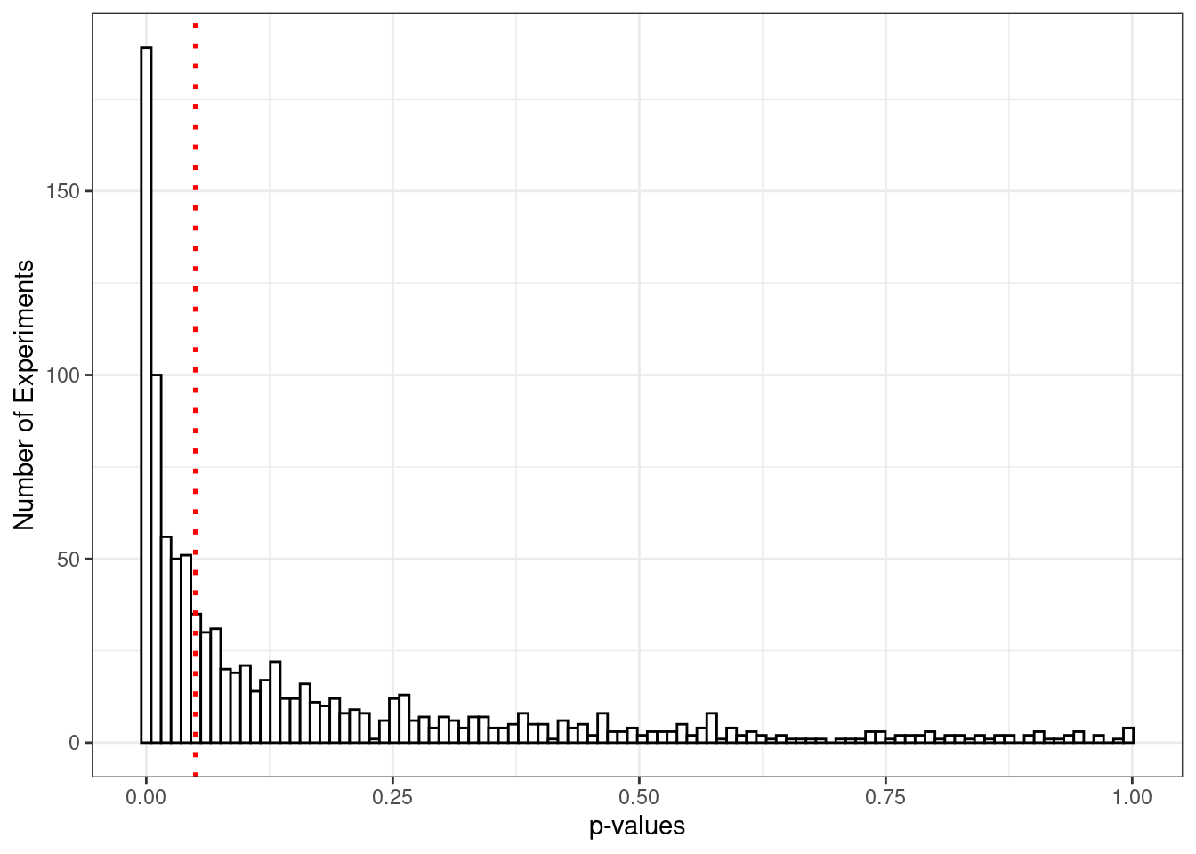
In addition to counting up how often your experiments come up statistically significant, you can directly observe the distribution of p-values you’re likely to get. The graph below shows that under these assumptions, you can get expect to get quite a few p-values in the 0.01 range, but that 80% will be below 0.05.
Code
library(ggplot2)bardf <- diag$simulations_dfggplot(bardf, aes(x = p.value)) +geom_histogram(fill ="white", color ="black", bins =100) +geom_vline(xintercept =0.05, color ="red", linetype ="dotted", size =1) +labs(x ="p-values", y ="Number of Experiments") +theme_bw()
7 7. How to Change your Design to Improve Your Power
When it comes to statistical power, the only thing that that’s under your control is the design of the experiment. As we’ve seen above, an obvious design choice is the number of subjects to include in the experiment. The more subjects, the higher the power.
However, the number of subjects is not the only design choice that has consequences for power. There are two broad classes of design choices that are especially important in this regard.
Choice of estimator. Are you using difference-in-means? Will you be doing some transformation, such as a logit or a probit? Will you be controlling for covariates? Will you be using some kind of robust standard error estimator? All of these choices will make a difference for the statistical significance of your results, and therefore for the power of your experiment. One easy way to think about this is to imagine what command you’ll be running in R or Stata after the experiment has come back; that’s your estimator!
Randomization Protocol. What kind of randomization will you be employing? Simple randomization gives all subjects an equal probability of being in the treatment group, and then performs a (possibly weighted) coin flip for each. Complete randomization is similar, but it ensures that exactly a certain number will be assigned to treatment. Block randomization is even more powerful — it ensures that a certain number within a subgroup will be assigned to treatment. A restricted random assignment rejects some random assignments based on some set of criteria — lack of balance perhaps. These various types of random assignment can dramatically increase the power of an experiment at no extra cost. Read up on randomization protocols here.
There are too many choices to cover in this short article, but check out the Simulation for Power Analysis code page for some ways to get started. But to give a flavor of the simulation approach, consider how you would conduct a power analysis if you wanted to include covariates in your analysis.
If the covariates you include as control variables are strongly related to the outcome, then you’ve dramatically increased the power of your experiment.Unfortunately, the extra power that comes with including control variables is very hard to capture in a compact formula. Almost none of the power formulas found in textbooks or floating around on the internet can provide guidance on what the inclusion of covariates will do for your power.
The answer is simulation.
Suppose we’re studying the effect of an educational intervention on income
Suppose we have good data on the relationship between two covariates and income: age and gender. In this economy, men earn more than women, and older people earn more than younger people.
Run a regression of income on age and gender and record the coefficients, using pre-existing survey data (better yet: use baseline data from future participants in your experiment!) *Generate fake covariate data — N total subjects, but broken up by age and gender in a way that reflects your experimental subject pool.
Generate fake control data — where the outcome is a function of age and gender according to your regression estimates
Hypothesize a treatment effect to generate fake treatment data
Run the experiment 10,000 times, and record how often, using a regression with controls, your experiment turns up significant.
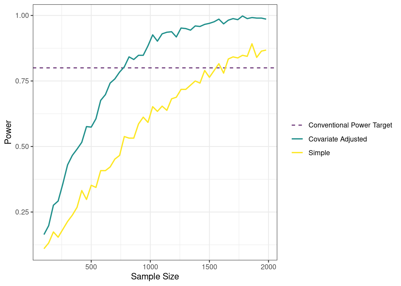
Here’s a graph that compares the power of an experiment that does control for background attributes to one that does not. The R-square of the regression relating income to age and gender is pretty high — around .66 — meaning that the covariates that we have gathered (generated) are highly predictive. For a rough comparison, sigma, the level of background noise that the unadjusted model is dealing with, is around 33. This graph shows that at any N, the covariate-adjusted model has more power — so much so that the unadjusted model would need 1500 subjects to achieve what the covariate-adjusted model can do with 500.
Code
ggplot(plotdf, aes(x = N, y = power, color = estimator)) +geom_hline(aes(color ="Conventional Power Target", yintercept =0.8 ), linetype ="dashed")+geom_line(size =0.75) +labs(x ="Sample Size", y ="Power", color ="") +scale_color_viridis_d()+theme_bw()
This approach doesn’t rely on a formula to come up with the probability of getting a statistically significant result: it relies on brute force! And because simulation lets you specify every step of the experimental design, you do a far more nuanced power analysis than simply considering the number of subjects.
8 8. Power Analysis for Multiple Treatments
Many experiments employ multiple treatments which are compared both to each other and to a control group. This added complication changes what we mean when we say the “power” of an experiment. In the single treatment group case, power is just the probability of getting a statistically significant result. In the multiple treatment case, it can mean a variety of things: A) the probability of at least one of the treatments turning up significant, B) the probability of all the treatments turning up significant (versus control) or C) the probability that the treatments will be ranked in the hypothesized order, and that those ranks will be statistically significant.
This question of multiple treatment arms is related to the problem of multiple comparisons. (See our guide on this topic for more details.) Standard significance testing is based on the premise that you’re conducting a single test for statistical significance, and the p-values derived from these tests reflect the probability under the null of seeing such a larger (or larger) treatment effect. If, however, you are conducting multiple tests, this probability is no longer correct. Within a suite of tests, the probability that at least one of the tests will turn up significant even when the true effect is zero is higher, essentially because you have more attempts. A commonly cited (if not commonly used) solution is to use the Bonferroni correction: specify the number of comparisons you will be making in advance, then divide your significance level (alpha) by that number.
If you are going to be using a Bonferroni correction, then standard power calculators will be more complicated to use: you’ll have to specify your Bonferroni-corrected alpha levels and calculate the power of each separate comparison. To calculate the probability that all the tests are significant, multiply all the separate powers together. To calculate the probability that at least one of the tests is significant, calculate the probability that none are, then subtract from one.
Or you can use simulation. An example of a power calculation done in R is available on the simulations page.
9 9. How to Think About Power for Clustered Designs
When an experiment has to assign whole groups of people to treatment rather than individually, we say that the experiment is clustered. This is common in educational experiments, where whole classrooms of children are assigned to treatment or control, or in development economics, where whole villages of individuals are assigned to treatment or control. (See our guide on cluster randomization for more details.)
As a general rule, clustering decreases your power. If you can avoid clustering your treatments, that is preferable for power. Unless you face concerns related to spillover, logistics, or ethics, take the variation down to the lowest level that you can.
The best case scenario for a cluster-level design is when which cluster a subject is in provides very little information about their outcomes. Suppose subjects were randomly assigned to clusters — the cluster wouldn’t help to predict outcomes at all. If the cluster is not predictive of the outcome, then we haven’t lost too much power to clustering.
Where clustering really causes trouble is when there is a strong relationship between the cluster and the outcome. To take the villages example, suppose that some villages are, as a whole, much richer than others. Then the clusters might be quite predictive of educational attainment. Clustering can reduce your effective sample size from the total number of individuals to the total number of clusters.
There are formulas that can help you understand the consequences of clustering — see Gelman and Hill (2006), page 447-449 for an extended discussion. While these formulas can be useful, they can also be quite cumbersome to work with. The core insight however is a simple one: you generally get more power from increasing the number of clusters than you do from increasing the number of subjects within clusters. Better to have 100 clusters with 10 subjects in each than 10 clusters with 100 subjects in each.
Again, a more flexible approach to power analysis when dealing with clusters is simulation. See the Declare Design library for block and cluster randomized experiments for some starter code. The DeclareDesign software aims to make simulations for power analysis (among many other tasks) easier. See also Gelman and Hill (2006), pages 450-453 for another simulation approach.
10 10. Good Power Analysis Makes Preregistration Easy
When you deal with power you focus on what you cannot control (noise) and what you can control (design). If you use the simulation approach to power analysis then you will be forced to imagine how your data will look and how you will handle it when it comes in. You will get a chance to specify all of your hunches and best guesses in advance, so that you can launch your experiments with clear expectations of what they can and cannot show. That’s some work but the good news is that if you really do it you are most of the way to putting together a comprehensive and registerable pre-analysis plan.