10 Randomization Inference Procedures with ri2

Randomization inference is a procedure for conducting hypothesis tests that takes explicit account of a study’s randomization procedure. See 10 things about Randomization Inference for more about the theory behind randomization inference. In this guide, we’ll see how to use the ri2 package for r to conduct 10 different analyses. This package was developed with funding from EGAP’s innaugural round of standards grants, which are aimed at projects designed to improve the quality of experimental research.

To illustrate what you can do with ri2, we’ll use some data from a hypothetical experiment involving 200 students in 20 schools. We’ll consider how to do randomization inference using a variety of different designs, including complete random assignment, block random assignment, cluster random assignment, and a multi-arm trial. You can check the kinds of random assignment methods guide for more on the varieties of random assignment.

Follow the links below to download the four datasets we’ll use in the examples:

1 Randomization inference for the Average Treatment Effect

We’ll start with the most common randomization inference task: testing an observed average treatment effect estimate against the sharp null hypothesis of no effect for any unit.

In ri2, you always “declare” the random assignment procedure so the computer knows how treatments were assigned. In the first design we’ll consider, exactly half of the 200 students were assigned to treatment using complete random assignment.

Code

library(ri2)
complete_dat <- read.csv("ri2_complete_dat.csv")
complete_dec <- declare_ra(N = 200)

Now all that remains is a call to conduct_ri. The sharp_hypothesis argument is set to 0 by default corresponding to the sharp null hypothesis of no effect for any unit. We can see the output using the summary and plot commands.

Code

sims <- 10000
ri_out <-
  conduct_ri(
    Y ~ Z,
    declaration = complete_dec,
    sharp_hypothesis = 0,
    data = complete_dat,
    sims = sims
  )
summary(ri_out)

  term estimate two_tailed_p_value
1    Z    41.98             0.1144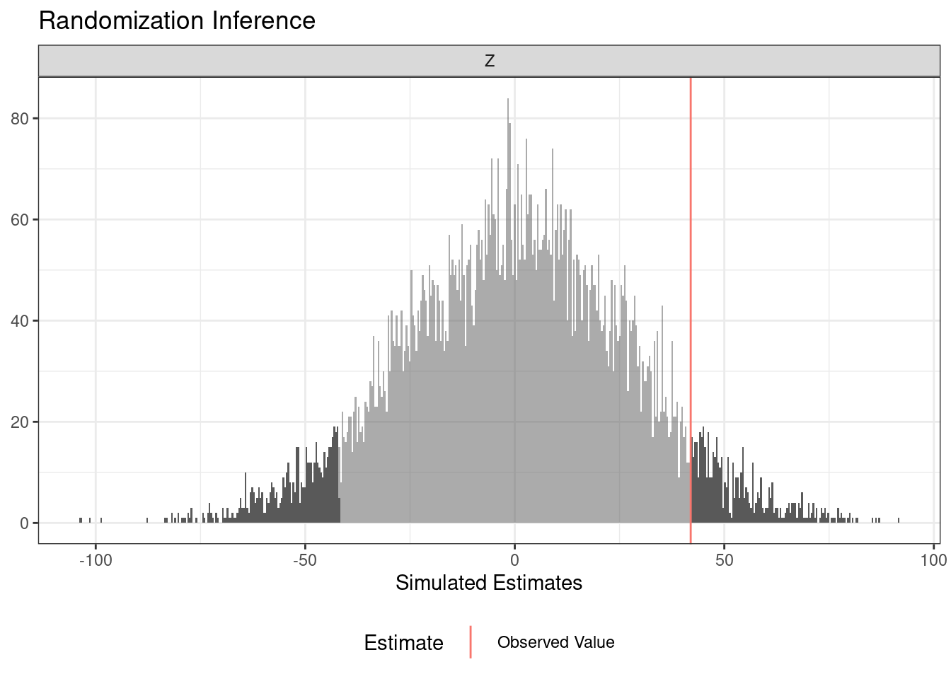

Code

plot(ri_out)

You can obtain one-sided p-values with a call to summary:

Code

summary(ri_out, p = "upper")

  term estimate upper_p_value
1    Z    41.98        0.0564

Code

summary(ri_out, p = "lower")

  term estimate lower_p_value
1    Z    41.98        0.9436

2 Randomization inference for alternative designs

The answer that ri2 produces depends deeply on the randomization procedure. The next example imagines that the treatment was blocked at the school level.

Code

blocked_dat <- read.csv("ri2_blocked_dat.csv")
blocked_dec <- declare_ra(blocks = blocked_dat$schools)
ri_out <-
  conduct_ri(
    Y ~ Z,
    declaration = blocked_dec,
    data = blocked_dat,
    sims = sims
  )
summary(ri_out)

  term estimate two_tailed_p_value
1    Z    91.98              2e-04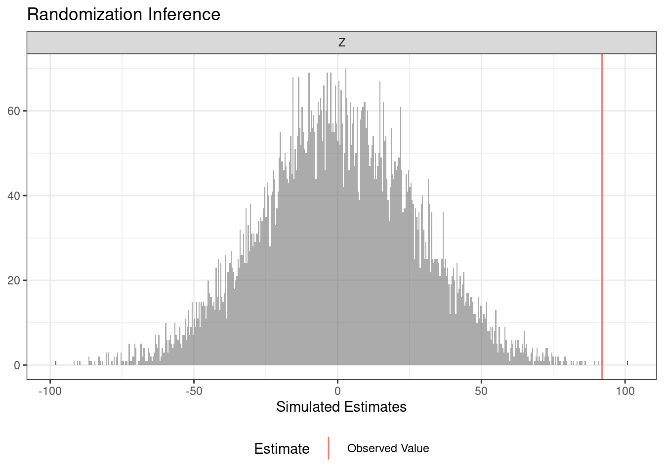

Code

plot(ri_out)

A very similar syntax accommodates a cluster randomized trial.

Code

clustered_dat <- read.csv("ri2_clustered_dat.csv")
clustered_dec <- declare_ra(clusters =  clustered_dat$schools)
ri_out <-
  conduct_ri(
    Y ~ Z,
    declaration = clustered_dec,
    data = clustered_dat,
    sims = sims
  )
summary(ri_out)

  term estimate two_tailed_p_value
1    Z    79.32             0.0111

Code

plot(ri_out)

3 Randomization inference with covariate adjustment

Covariate adjustment can often produce large gains in precision. To analyze an experiment with covariate adjustment, simply include the covariates in the formula argument of conduct_ri:

Code

complete_dec <- declare_ra(N = 200)
ri_out <-
  conduct_ri(
    Y ~ Z + PSAT,
    declaration = complete_dec,
    data = complete_dat,
    sims = sims
  )
summary(ri_out)

  term estimate two_tailed_p_value
1    Z 59.27132                  0

Code

plot(ri_out)

4 Randomization inference for a balance test

You can use randomization inference to conduct a balance test (or randomization check). In this case, we write a function of data that return some balance statistic (the F-statistic from a regression of the treatment assignment on two covariates).

Code

balance_fun <- function(data) {
  summary(lm(Z ~ professionalism + PSAT, data = data))$f[1]
}
ri_out <-
  conduct_ri(
    test_function = balance_fun,
    declaration = complete_dec,
    data = complete_dat,
    sims = sims
  )

Warning in data.frame(est_sim = test_stat_sim, est_obs = test_stat_obs, : row
names were found from a short variable and have been discarded

Code

summary(ri_out)

                   term  estimate two_tailed_p_value
1 Custom Test Statistic 0.2924994             0.7489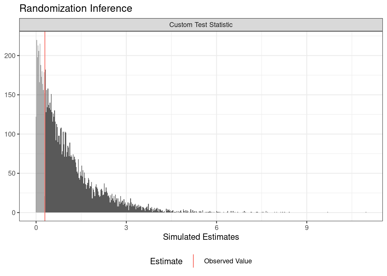

Code

plot(ri_out)

5 Randomization inference for treatment effect heterogeneity by subgroups

You can assess whether the treatment engenders different treatment effects among distinct subgroups by comparing the model fit (using an F-statistic) of two nested models:

A regression of the outcome on the treatment assignment and the subgroup indicator
A regression of the outcome on the treatment assignment, subgroup indicator, and their interaction

The null hypothesis we’re testing against in this example is the sharp hypothesis that the true treatment effect for each unit is the observed average treatment effect, i.e., that effects are constant.

Code

ate_obs <- with(complete_dat, mean(Y[Z == 1]) - mean(Y[Z == 0]))
ri_out <-
    conduct_ri(
      model_1 = Y ~ Z + high_quality,
      model_2 = Y ~ Z + high_quality + Z * high_quality,
      declaration = complete_dec,
      sharp_hypothesis = ate_obs,
      data = complete_dat, 
      sims = sims
    )
summary(ri_out)

         term estimate two_tailed_p_value
1 F-statistic 1.095294             0.7015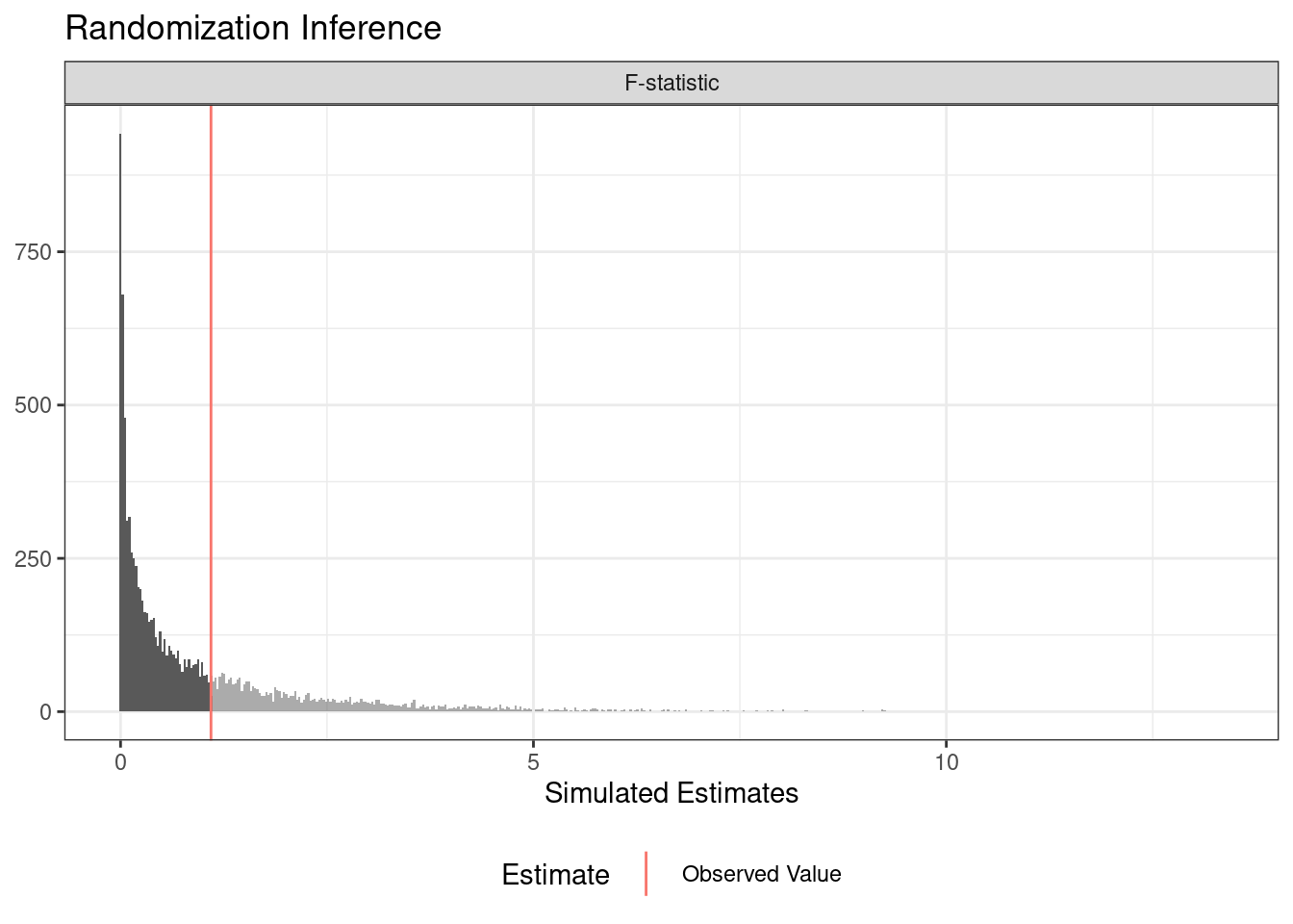

Code

plot(ri_out)

6 Randomization inference for unmodeled treatment effect heterogeneity

Another way to investigate treatment effect heterogeneity is to consider whether the variance in the treatment and control groups are different. We can therefore test whether the difference-in-variances is larger in magnitude than what we would expect under the sharp null hypothesis of no effect for any unit.

Code

d_i_v <- function(dat) {
    with(dat, var(Y[Z == 1]) - var(Y[Z == 0]))
  }
ri_out <-
    conduct_ri(
      test_function = d_i_v,
      declaration = complete_dec,
      data = complete_dat, 
      sims = sims
    )
summary(ri_out)

                   term  estimate two_tailed_p_value
1 Custom Test Statistic -8408.684             0.2824

Code

plot(ri_out)

7 Randomization inference for multi-arm trials

In a three-arm trial, the research might wish to compare each treatment to control separately. To do this, we must change the null hypothesis in a subtle way: we are going to assume the sharp null for each pairwise comparison. For example, when comparing treatment 1 to control, we exclude the subjects assigned to treatment 2 and pretend we simply have a two arm trial conducted among the subjects assigned to control and treatment 1.

Code

three_arm_dat <- read.csv("ri2_three_arm_dat.csv")
three_arm_dec <- declare_ra(N = 200, 
                            conditions = c("Control", "Treatment 1", "Treatment 2"))
ri_out <-
    conduct_ri(
      formula = Y ~ Z,
      declaration = three_arm_dec,
      data = three_arm_dat,
      sims = sims
    )
summary(ri_out)

          term  estimate two_tailed_p_value
1 ZTreatment 1  26.72546                 NA
2 ZTreatment 2 -48.52827                 NA

Code

## plot(ri_out)

8 Randomization inference for joint significance

In that same three-arm trial that compares two treatments to a control, we might be interested in testing whether, jointly, the treatments appear to change outcomes relative to the control. This is analogous to a joint F-test, conducted via randomization inference. We assume the sharp null that a unit would express their observed outcome in any of the three conditions.

Code

F_statistic <- function(data) {
  summary(lm(Y ~ Z, data = data))$f[1]
}
ri_out <-
   conduct_ri(
     test_function = F_statistic,
     declaration = three_arm_dec,
     data = three_arm_dat,
     sims = sims
   )

Warning in data.frame(est_sim = test_stat_sim, est_obs = test_stat_obs, : row
names were found from a short variable and have been discarded

Code

summary(ri_out)

                   term estimate two_tailed_p_value
1 Custom Test Statistic 2.802927             0.0664

Code

plot(ri_out)

9 Randomization inference under noncompliance

Some experiments encounter noncompliance, the slippage between treatment as assigned and treatment as delivered. The Complier Average Causal Effect (\(CACE\)) can be shown (under standard assumptions plus monotonicity) to be the ratio of the effect of assignment on the outcome – the “Intention-to-Treat” (\(ITT_y\)) and the effect of assignment on treatment receipt the (\(ITT_D\)). (The \(CACE\) is also called Local Average Treatment Effect. See our guide 10 Things to Know About the Local Average Treatment Effect for more details.) Because the \(CACE\) is just a rescaled, \(ITT_y\), a hypothesis test with respect to the \(ITT_y\) is a valid test for the \(CACE\). In practice, researchers can simply conduct a randomization inference test exactly as they would for the ATE, ignoring noncompliance altogether.

Code

ITT_y = with(complete_dat, mean(Y[Z == 1]) - mean(Y[Z == 0])) 
ITT_d = with(complete_dat, mean(D[Z == 1]) - mean(D[Z == 0])) 
CACE <- ITT_y / ITT_d
           
ri_out <-
  conduct_ri(
    Y ~ Z, # notice we do inference on the ITT_y
    declaration = complete_dec,
    data = complete_dat,
    sims = sims
  )
summary(ri_out)

  term estimate two_tailed_p_value
1    Z    41.98             0.1156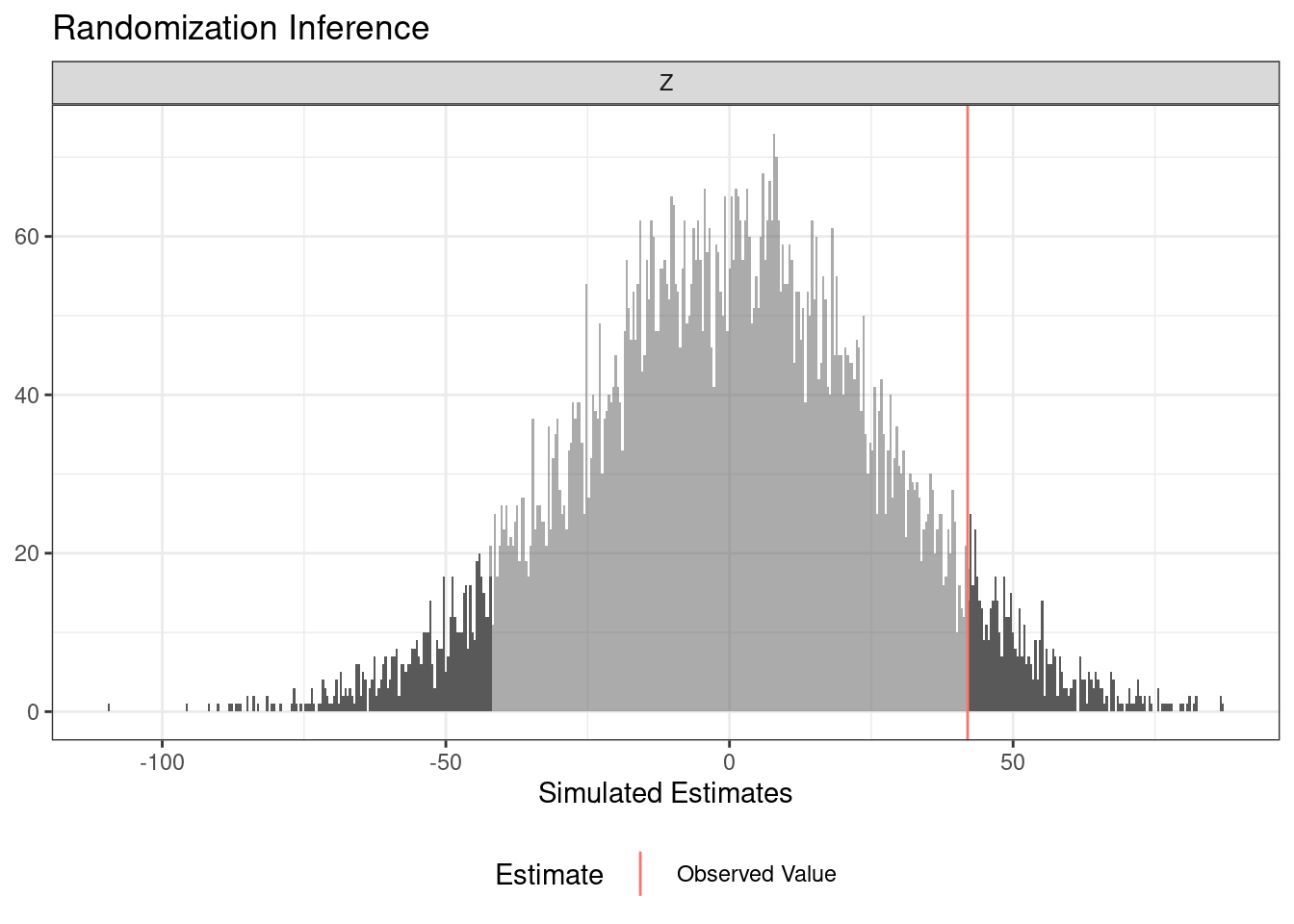

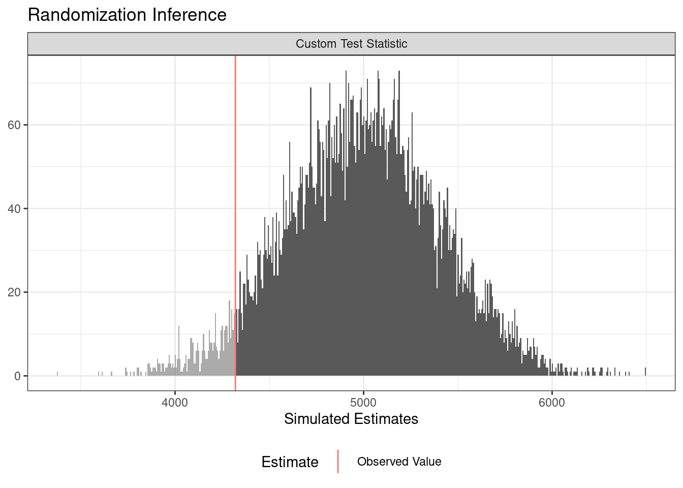
Code

plot(ri_out)

10 Randomization inference for arbitrary test statistics

ri2 can accommodate any scalar test statistic. A favorite among some analysts is the Wilcox rank-sum statistic, which can be extracted from the wilcox.test() function:

Code

wilcox_fun <- function(data){
  wilcox_out <- with(data, wilcox.test(Y ~ Z))
  wilcox_out$statistic
}
ri_out <-
  conduct_ri(
    test_function = wilcox_fun,
    declaration = complete_dec,
    data = complete_dat,
    sims = sims
  )

Warning in data.frame(est_sim = test_stat_sim, est_obs = test_stat_obs, : row
names were found from a short variable and have been discarded

Code

summary(ri_out)

                   term estimate two_tailed_p_value
1 Custom Test Statistic     4320             0.9565

Code

plot(ri_out)